
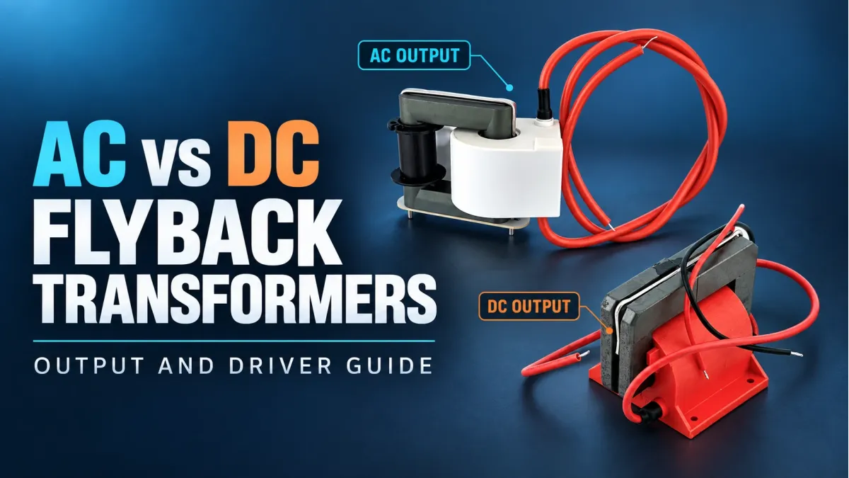
The choice between an AC flyback transformer and a DC flyback transformer starts with the output your circuit needs. An AC flyback provides a high-voltage output without an internal rectifier, allowing the voltage to reverse polarity with suitable drive. A DC flyback adds an internal rectifier, giving the external output a defined polarity. Choose AC if the load needs alternating voltage, or if you want to add your own rectifier or high-voltage multiplier. Choose DC if the built-in rectified output and its ground connection suit the application.
That output choice does not determine how the primary is powered. Both types need a flyback transformer driver that switches the voltage applied to the primary winding; neither is intended for a direct connection to steady DC or 50/60 Hz mains. A single MOSFET switch, a push-pull driver, a half-bridge and a full-bridge provide different ways to produce this changing voltage. In this guide, we will compare their operation and explain how to match the driver to the winding and load, using high-voltage flyback transformers from our High Voltage Experimental (HVE) AC and DC flyback range.
In this guide: AC versus DC output · Winding capacitance and resonance · Comparing driver circuits · Matching the driver · Choosing HVE products · Voltage multipliers · Common questions
Is a flyback transformer AC or DC?
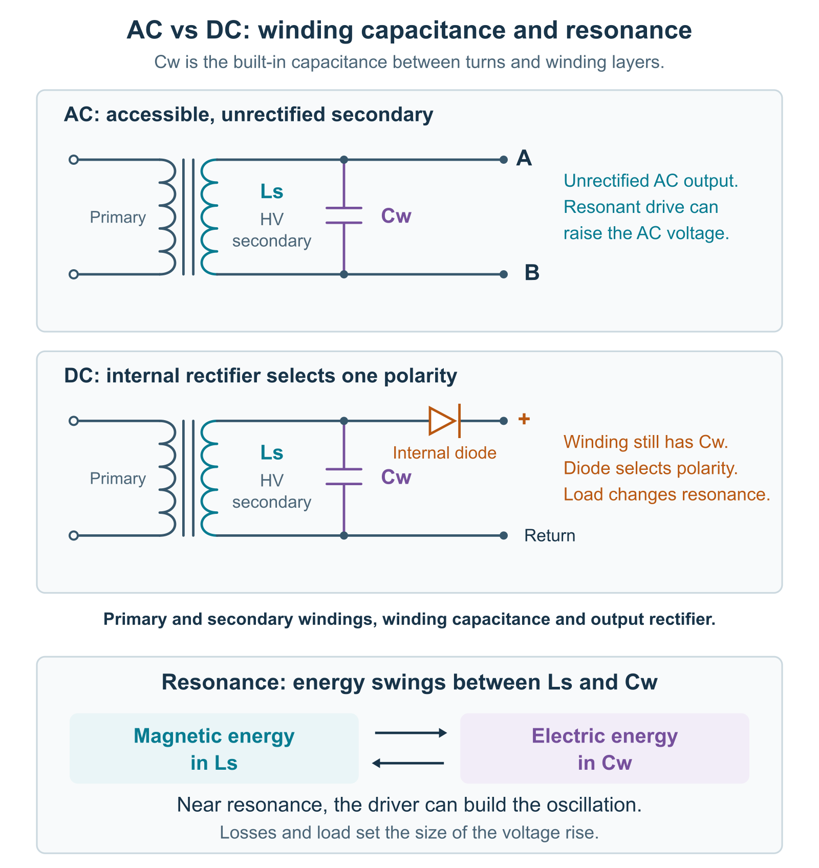
To understand the AC/DC distinction, consider the secondary winding in Figure 1. The winding produces voltage as the magnetic flux in the core changes. An AC-output transformer connects this winding to the output without an internal diode, so a suitable driver can produce both positive and negative output voltage. In a DC-output transformer, an internal rectifier passes current in one direction and gives the external output a defined polarity. The AC or DC label therefore describes the high-voltage output, while the supply feeding the driver can be DC in either case.
| Question | AC-output transformer | Internally rectified DC transformer |
|---|---|---|
| What is available at the output? | Voltage without internal rectification. It can reverse polarity with suitable drive. | Rectified voltage with a defined output polarity. |
| Is the waveform automatically smooth? | No. The driver, resonance and load determine the shape. | No. The output can contain pulses and ripple. |
| When is it useful? | AC loads, external rectification and high-voltage multipliers. | Loads that need the output polarity provided by the model. |
| Can the output float? | Yes, in many cases it can. Check the winding connections and insulation specification. | Check the internal winding and rectifier connections. A shared connection with the primary can set the reference point for the output voltage. |
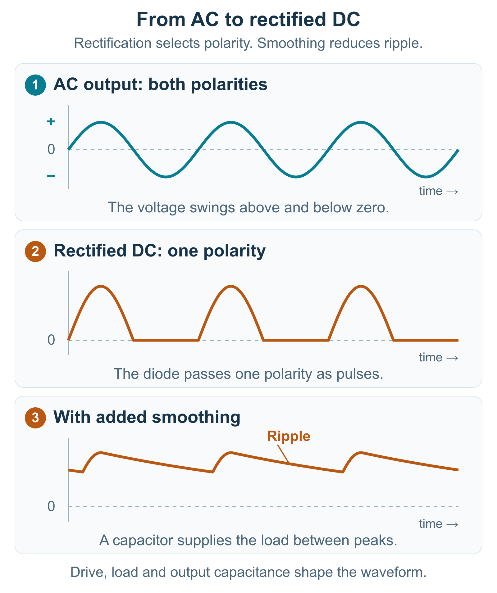
The rectifier gives the output one polarity, but pulses and ripple can remain between switching cycles. Adding output capacitance helps hold the voltage between pulses and reduces this ripple. If the application also needs a stable output voltage as the load changes, a feedback circuit can adjust the drive to maintain the required level. These functions serve different purposes, so the capacitance and control circuitry you need depend on how the load will use the DC output.
The output connection also matters when choosing a model. In the HVE 30 kV DC flyback transformer, the secondary is internally connected to the primary. Its output is positive relative to the specified ground reference, and this common connection sets the output reference and polarity. If your circuit needs a different reference or external control over rectification, an AC-output transformer provides that flexibility, subject to its winding connections and insulation limits.
Winding capacitance and resonant operation
Figure 1 also shows a property shared by both transformer types: winding capacitance. The turns and layers of a high-voltage winding are close together, with insulation between them, so the neighbouring conductors behave like small capacitor plates. Their combined effect is represented by \(C_{\mathrm{w}}\) across the winding. The winding stores magnetic energy through its inductance, while this capacitance stores electric energy. Energy can move back and forth between the two forms, producing an oscillation. Analog Devices' LC-resonance tutorial explains this energy exchange and winding self-resonance.
A driver operating near a suitable resonance can add energy at the right point on successive cycles, much like pushing a swing in time with its motion. This allows the winding voltage to rise above the value expected from the turns ratio alone. The energy still comes from the driver; resonance provides a way for it to build up in the circuit. Winding and core losses limit the voltage rise, as does power taken by the load. With an AC flyback, the alternating winding voltage is directly available at the output, making this behaviour useful for resonant operation.
The resonant frequency depends on the inductance and capacitance involved. If one resonant mode dominates the response, a useful estimate is:
\[f_0 \approx \frac{1}{2\pi\sqrt{L_{\mathrm{eff}}C_{\mathrm{eff}}}}\]
Here, \(L_{\mathrm{eff}}\) is the effective inductance and \(C_{\mathrm{eff}}\) is the effective capacitance, both referred to the same winding. The primary connections and magnetic coupling determine how the transformer's magnetizing and leakage inductances contribute, as shown in TI's discussion of transformer resonance. The capacitance includes the winding itself and contributions from connected cables, probes or added capacitors. For the same mode and inductance, increasing capacitance lowers the resonant frequency. This means that adding a load or measurement probe can change the frequency you need to use; Coilcraft's self-resonance note explains the relationship.
A DC flyback also has winding capacitance, but its internal rectifier changes how the load draws energy from the winding. Its resonant response can therefore differ from that of an unrectified AC transformer. Changing the driver can change the response, but it cannot remove the rectifier or make both winding polarities available at the external output. With the output construction understood, the next question is how the driver applies voltage to the primary.
Comparing flyback transformer drivers
Single-switch, push-pull, half-bridge and full-bridge drivers can all use MOSFETs. Each arrangement connects the switches differently to apply voltage to the primary. The DC bus voltage is the supply voltage for the power stage. The voltage across the primary depends on the switching arrangement and the winding's return connection, while the transformer produces the high-voltage secondary output. We will use these terms in the examples below to show how a given supply voltage produces different primary waveforms.
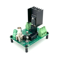
A MOSFET switch board: one controlled switch
A single-switch board provides a building block for a power stage of your own design. Our HVE TO-247-4 MOSFET switch board, for example, contains one power MOSFET and its gate-drive electronics. The gate driver turns the MOSFET on and off in response to a control signal, while you provide the surrounding power circuit. The board's 12 V auxiliary input powers the gate-drive electronics; transformer power passes through the power circuit connected to the MOSFET.
Figure 2 shows how that switch can be used in a conventional flyback circuit. The primary is connected between the DC supply and the MOSFET. When the MOSFET turns on, primary current rises and the transformer stores magnetic energy. When the MOSFET turns off, the winding voltage reverses and the secondary rectifier conducts, transferring energy to the load. The transformer, winding polarity, rectifier and switching timing must all support this sequence. Analog Devices' flyback reference design illustrates this operating principle.
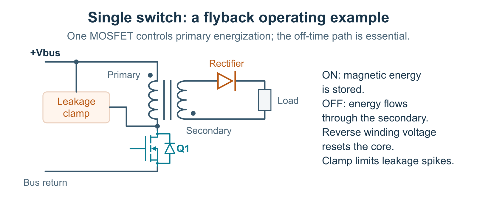
During off-time, energy passes to the secondary and the reverse primary voltage resets the core for the next cycle. The MOSFET must withstand the DC bus voltage plus the secondary voltage reflected back to the primary. Leakage inductance produces an additional voltage spike when the MOSFET turns off, and a clamp or snubber limits this spike. Its operating level must still allow the reverse winding voltage needed for energy transfer and core reset. TI's flyback-clamp discussion explains how this leakage energy is handled.
This arrangement is useful when you want to choose the pulse timing and design the energy-transfer circuit yourself. The surrounding circuit provides the required timing, current limiting and output control, while the board provides the controlled switch. For resonant operation, you also need the appropriate resonant components and drive conditions. Push-pull and bridge drivers provide other ways to drive the core in both magnetic directions, as the next examples show.
Push-pull: two switches and a centre-tapped primary
A push-pull driver uses a primary winding with a connection at its midpoint, called a centre tap. In Figure 3, this tap connects directly to the positive DC supply, and two MOSFETs take turns connecting the outer ends to the supply return. Each switch powers one half of the winding, producing magnetic flux changes in opposite directions. Both MOSFET sources connect to the supply return, which makes their gate-drive circuits simpler.
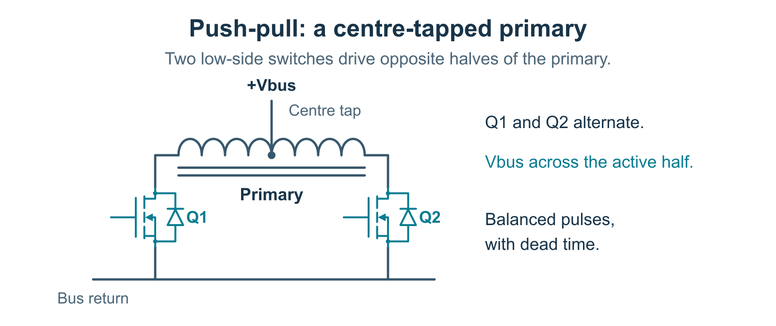
During each drive pulse, approximately the full bus voltage is applied across the active half of the primary. The MOSFET that is off sees about twice the bus voltage, plus switching spikes. The two winding halves need equal turns, and the drive pulses must keep the magnetic flux balanced to avoid saturation. This circuit has no capacitor midpoint to help restore that balance, so the driver needs suitable timing and current protection. TI's comparison of push-pull and bridge circuits explains these requirements.
A push-pull driver with an external controller can provide adjustable frequency and pulse width. A short interval with both switches off prevents their drive pulses from overlapping. Controllers such as the LTC3721-1 also provide current limiting for each switching cycle. These controls let you adjust the drive to suit the transformer and load.
A half-bridge: two switches and a defined primary return
A half-bridge uses two switches in one leg. The high-side switch connects the switching node to the positive DC bus, and the low-side switch connects it to the negative bus. In Figure 4, one end of the primary connects to this switching node and the other to the midpoint of the split DC bus. The voltage across the winding is the difference between these two connections. With a balanced supply and ideal switching, it therefore alternates between \(+\frac{V_{\mathrm{bus}}}{2}\) and \(-\frac{V_{\mathrm{bus}}}{2}\).
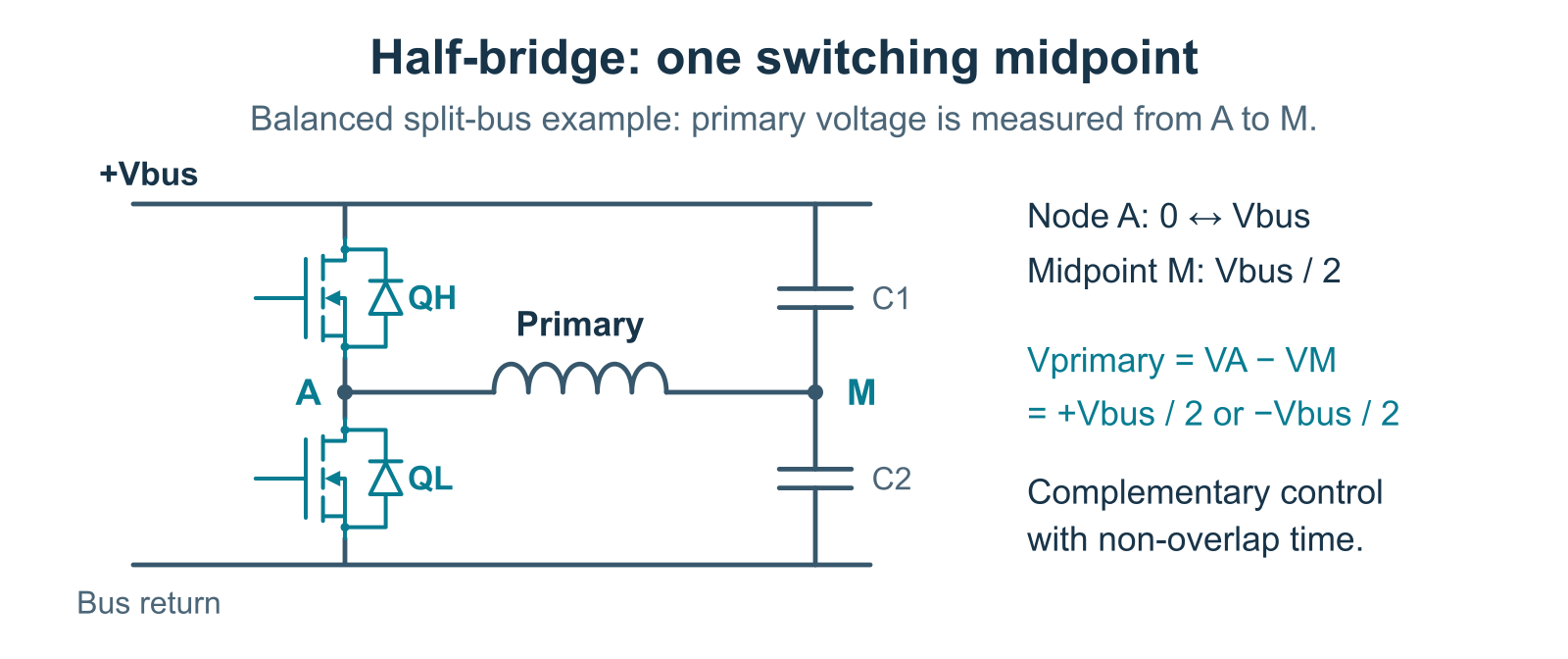
Applying both polarities makes the half-bridge useful for AC and resonant transformer operation. Our HVE 80 V half-bridge amplifier provides an output of ± half its supply voltage and accepts an external square-wave control signal. A function generator or suitable logic source sets the switching frequency and duty cycle, which is the fraction of a cycle for which the signal is active. This lets you adjust the drive with the intended transformer and load connected. The timing in a typical self-oscillating ZVS module follows its resonant circuit, as we explain later under ZVS drivers.
In the half-bridge, switch timing must meet two requirements. First, the switches in each leg must not conduct together, because this would short the supply. Dead time provides a short interval with both switches off, as illustrated in TI's half-bridge gate-driver reference design. Second, the positive and negative drive intervals must maintain magnetic balance in the transformer. The winding must also support the voltage and pulse duration applied by the driver. The section on voltage-time limits explains how to check this.
A full-bridge: four switches reverse the primary connection
A full-bridge, also called an H-bridge, extends this approach to four switches arranged in two legs. Instead of connecting the primary to one switching node and a bus midpoint, it connects the primary between the switching nodes of both legs. One diagonal switch pair makes node A positive relative to node B, and the other pair reverses this voltage. Depending on the switching pattern, the bridge can also provide a zero-voltage state. Figure 5 shows these connections with an optional capacitor in series with the primary.
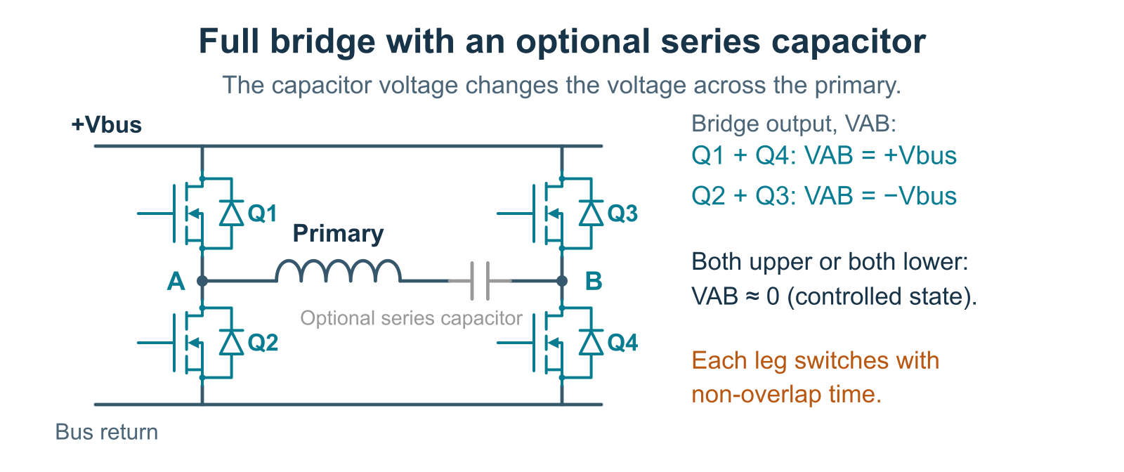
With the primary connected directly between A and B, its ideal voltage alternates between \(+V_{\mathrm{bus}}\) and \(-V_{\mathrm{bus}}\). At the same bus voltage, this gives twice the primary voltage amplitude of the balanced half-bridge example. The output power you can obtain also depends on the transformer and load, so the higher primary voltage must suit their operating limits. Applying twice the voltage to the same winding for the same time doubles its magnetic flux change. This can drive the core into saturation, where primary current can rise sharply.
How the capacitors reduce primary drive and help prevent saturation
In the split-capacitor half-bridge shown in Figure 4, one end of the primary connects to the switches and the other to the capacitor midpoint. During a positive drive interval, current flowing into the midpoint raises its voltage. This reduces the voltage across the primary, even while the high-side switch remains on. For example, with a 40 V bus, a midpoint rise from 20 V to 25 V reduces the primary voltage from 20 V to 15 V. As charge is transferred, less voltage is available to drive further primary current.
The midpoint movement also gives the split-capacitor half-bridge a built-in balancing effect that helps prevent saturation caused by unequal drive intervals. With suitable voltage-driven switching, an interval that is too long shifts the capacitor voltages so that less primary voltage is applied in that direction and more is applied in the other direction. This helps balance the magnetization in the two directions and keeps the core's magnetic flux from gradually drifting towards saturation. A directly connected full-bridge relies on its drive timing or control circuitry to maintain that balance. TI's half-bridge application note explains this capacitor balancing effect.
The capacitor values determine how much their voltages change for a given amount of charge. This follows \(Q = C\,\Delta V\), where \(C\) is capacitance and \(\Delta V\) is the voltage change. With fixed DC bus rails, the capacitance seen at the midpoint is the sum of the two split capacitors. If each capacitor is 1.5 µF, the effective midpoint capacitance is 3 µF, and a 10 V midpoint shift corresponds to 30 µC of net charge. Larger capacitors give a smaller voltage change for the same transferred charge.
In a full-bridge without the optional series capacitor, the switches connect both ends of the primary to the supply rails. With a steady 40 V bus, the bridge can keep applying 40 V across the winding throughout its commanded on-time. It has no capacitor midpoint that moves as charge is transferred, so the applied voltage remains constant during that interval.
Adding a capacitor in series with the full-bridge primary gives a similar effect to the midpoint capacitors. All primary current flows through this capacitor, changing its voltage as charge is transferred. When that voltage opposes the bridge output, less voltage remains across the winding and the current rises more slowly. The capacitor also helps compensate for small differences between positive and negative drive pulses, reducing the risk of the core's magnetic flux gradually drifting towards saturation. It is often called a DC-blocking capacitor because it prevents a steady DC current through the winding. TI's full-bridge design guide describes this arrangement.
The capacitance determines how strongly this affects the drive. A large capacitor may block DC while allowing only a small voltage change during each pulse. A smaller capacitor changes voltage more quickly for the same transferred charge, but it also changes the circuit's resonance. Depending on the switching frequency and load, this can increase current and winding voltage, so the value must suit the transformer and operating conditions.
Either bridge can still saturate if the applied voltage and on-time are too large for the winding. High current can also develop during overload or resonant operation, as discussed in ST's resonant half-bridge application note. For a defined peak-current limit, a current-sense circuit can shorten or stop the drive when the chosen level is reached. In a split-capacitor half-bridge, the protection scheme must also maintain balanced drive intervals and capacitor voltages. Current protection can be included in single-switch, push-pull, half-bridge and full-bridge designs.
The full-bridge gives you more control over the primary waveform, although it needs more switches and coordinated timing. A back-to-back bidirectional MOSFET switch is useful when you need to open or close a current path in either direction. The full-bridge in Figure 5 uses its two switching legs to reverse the voltage between A and B. The table below compares the primary voltages and the main design requirements for these circuits.
| Driver | Primary excitation | Main design responsibility |
|---|---|---|
| Single MOSFET, flyback example | About \(+V_{\mathrm{bus}}\) during on-time. The circuit sets the reverse voltage during reset. | Energy-transfer path, core reset, current limiting and switch voltage spikes. |
| Push-pull with a centre-tapped primary | Approximately \(V_{\mathrm{bus}}\) across the active half of the primary. The two halves are driven alternately. | Equal winding halves, balanced drive pulses, dead time, current limiting and switch voltage spikes. |
| Balanced half-bridge | Approximately \(\pm\frac{V_{\mathrm{bus}}}{2}\). | Primary return connection, switch timing, dead time and magnetic balance. |
| Full-bridge with a direct primary connection | Approximately \(\pm V_{\mathrm{bus}}\); zero states are possible. | Timing for both switch legs, magnetic balance and primary voltage-time limits. |
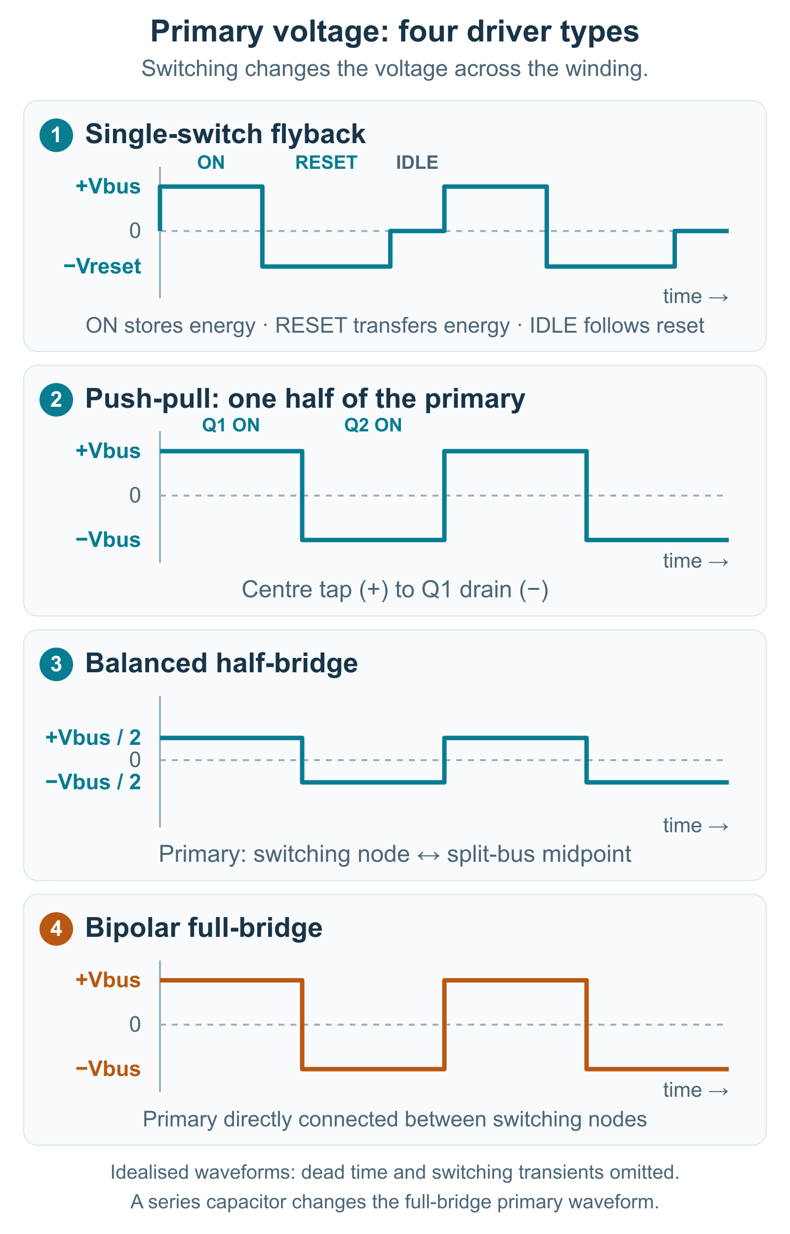
For a numerical example, consider a 40 V DC bus. A push-pull driver applies approximately 40 V across the active half of its primary. A balanced half-bridge applies approximately +20 V and −20 V across the primary, while a full-bridge with a direct primary connection can apply +40 V and −40 V. These values describe the ideal connections shown in the diagrams; coupling components, a resonant network and the load can change the actual winding voltage. TI's power-topology comparison explains the basic difference. Figure 6 compares all four drivers, with the push-pull voltage measured across one half of the primary. The practical question is whether the winding can support the voltage and timing produced by the chosen driver.
Why push-pull and bridge drivers suit an AC flyback transformer
A push-pull driver uses the two halves of its primary to produce opposite magnetic flux changes. Half-bridges and full-bridges do this by reversing the voltage across one winding. This is called bipolar drive. With an AC-output transformer and a suitable load, these drivers can supply energy and transfer power to the secondary during both halves of the cycle. The driver can therefore keep adding energy as the voltage changes polarity. In the single-switch flyback example, energy is stored while the MOSFET is on and transferred to the secondary after it turns off.
Using both halves of the cycle for power transfer can allow more power through a suitable AC transformer than the single-switch flyback arrangement. The achievable power still depends on the winding, core, switching frequency, load and temperature limits. Near resonance, an externally controlled push-pull or bridge driver also lets you adjust the frequency and drive intervals to suit the transformer while maintaining magnetic balance. A single switch can also drive a resonant circuit, but its operation depends on the surrounding components.
How to match a flyback transformer driver
Check the primary winding and voltage-time limit
When matching a driver to the primary, check the winding's turns, inductance and core gap alongside the intended bus voltage and pulse duration. These properties affect how current and magnetic flux develop during each pulse. A higher voltage or a longer pulse produces a larger change in core flux density, so both voltage and pulse duration belong in the compatibility check. Ignoring winding resistance and leakage voltage drops, this relationship can be written as:
\[\Delta B \approx \frac{1}{N_{\mathrm{p}}A_{\mathrm{e}}}\int v_{\mathrm{p}}(t)\,\mathrm{d}t\]
In this expression, \(\Delta B\) is the change in core flux density, \(N_{\mathrm{p}}\) is the number of turns in the winding section being driven, and \(A_{\mathrm{e}}\) is the effective core area. The integral adds up the primary voltage over time. For push-pull, use the voltage across one half of the primary and the number of turns in that half. During repeated operation, the positive and negative induced voltage-time areas must balance over each complete cycle; otherwise, the flux can drift towards saturation. In a single-switch flyback, the off-time reset provides this balance. Coilcraft's transformer-design guide explains why voltage, frequency and primary turns must be considered together.
The primary connections must suit the driver as well. If a driver needs a centre tap, the primary must provide that connection; a bridge can drive a winding with two terminals. A monitoring winding provides a signal for measurement or feedback and should be connected to the appropriate monitoring input. Checking how each winding is used will help you choose a driver that matches both the transformer's connections and its operating requirements.
Match frequency to the loaded transformer
Once the winding and voltage are suitable, choose a frequency supported by the driver and the transformer under load. Our half-bridge boards can switch at frequencies up to 500 kHz. The transformer's useful operating frequency depends on its winding and load, so check the transformer and driver specifications together when choosing the operating frequency.
The load is part of this frequency choice because it changes the transformer's resonant response. Adding a multiplier, cable or probe changes the capacitance and loading seen by the winding. The frequency that gives the highest unloaded voltage may therefore differ from the best operating point under load. Adjust the frequency with the intended circuit connected, rather than treating an unloaded voltage peak as the final setting.
Understand what “ZVS flyback driver” means
ZVS means zero-voltage switching. A MOSFET operating with ZVS turns on when the voltage across it is close to zero, which can reduce switching losses. Half-bridges and full-bridges can use this method when the circuit conditions allow the MOSFETs to turn on at that point. Whether this happens depends on the drive conditions and resonant network, so ZVS needs to be considered together with the chosen transformer and load.
Many small modules sold as “ZVS flyback drivers” use a self-oscillating, two-MOSFET circuit, commonly called a Mazzilli driver. Its MOSFETs take turns conducting, normally for approximately half of each cycle, giving about 50% duty cycle in balanced operation. The switching frequency follows the resonant output stage and depends on the primary inductance, resonant capacitor and connected transformer and load. These modules usually have no independent controls for frequency or duty cycle. To change their operating frequency, you change the winding or resonant components; the load can change it further. An externally controlled push-pull or bridge driver gives you more freedom to choose and adjust the timing.
The fixed switching pattern also limits how you control power. A basic ZVS module cannot independently shorten its drive pulses while keeping the same operating frequency. Lowering the DC supply within the module's operating range can reduce power, but it also reduces the available high voltage and may prevent a discharge from starting. For plasma experiments that need high voltage with low average power, an externally controlled driver with adjustable pulse width or burst control gives you more control over the energy delivered to the discharge.
Burst control runs the AC drive for a group of cycles, then pauses it. The burst duty cycle sets the fraction of time the whole drive is active; each MOSFET can still operate at about 50% duty during those active cycles. Increasing the off-time can reduce average power while allowing a high voltage during each burst, and the pauses give the gas time to cool. A basic self-oscillating ZVS module would need additional control designed for reliable stopping and restarting to provide this function.
When choosing a self-oscillating ZVS driver, check its primary connections, resonant components, supply range, current limits and startup behaviour. A change in transformer or load can alter the resonant currents and the voltage present when a MOSFET turns on. To check for ZVS, measure the drain-to-source voltage and gate signal of each MOSFET. The drain-to-source voltage should be close to zero when the gate signal turns the MOSFET on. A sine-shaped secondary waveform does not show whether this condition is met. TI's UCC256303 resonant-controller datasheet describes how switching conditions are controlled in its converter design.
Choosing an HVE transformer and driver
These checks provide a practical order for choosing components: start with the required output, select a suitable winding, then match the driver's voltage, timing and frequency. The models from our range below illustrate how the output construction and winding options lead to different choices. Read these ratings together with the intended load and operating conditions.
The unloaded resonance values below apply with the core assembled without a gap and no load connected to the secondary.
| Product | Choose it for | Unloaded resonance |
|---|---|---|
| 15 kV AC flyback transformer | For moderate-voltage setups with limited space. AC output, 2,400-turn secondary; wind your own primary. | ≈40 kHz |
| 25 kV AC flyback transformer | AC output with a choice of secondary windings. Wind your own primary or select a prewound primary. | 2,400 turns: ≈46 kHz 1,000 turns: ≈110 kHz 560 turns: ≈195 kHz |
| 30 kV DC flyback transformer | Positive DC output with a shared primary/secondary connection. Typical input: 12–24 V. | Not specified. |
The 25 kV model has an optional primary with a 40-turn power winding and a 4-turn monitor winding. For the AC models, check the primary winding and operation under load. For the DC model, check the primary waveform, shared connection and insulation limits.
Use these unloaded resonance values as a starting point when setting up the driver. Adding a core gap or connecting a multiplier, cable, probe or other load can change the resonant frequency, so tune the transformer with the intended circuit connected.
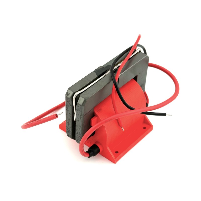
When comparing the AC models, pay attention to the voltage convention. We specify the AC models by their peak output voltage: 15 kV corresponds to 30 kV peak-to-peak, and 25 kV corresponds to 50 kV peak-to-peak. These ratings are not RMS values. Peak-to-peak voltage is the difference between the highest and lowest instantaneous values. For a symmetric sine wave, \(V_{\mathrm{RMS}} = \frac{V_{\mathrm{peak}}}{\sqrt{2}}\). Other waveforms, including rectified pulses, need a calculation appropriate to their shape.
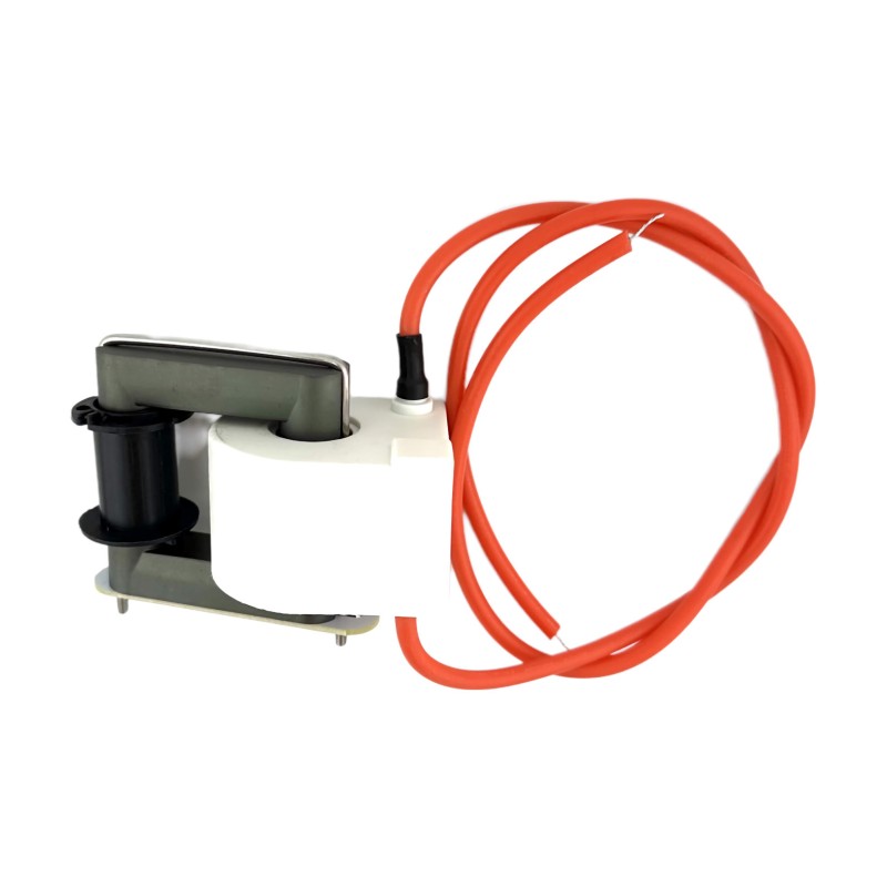
Our DC transformer is rated for an output up to 30 kV, while its supplied output lead has an insulation rating of 20 kV. When designing the high-voltage connection, check the lead rating and the required insulation and spacing alongside the transformer's operating conditions. The voltage you intend to use must be suitable for the wiring and connections as well as the transformer.
For externally controlled operation, our 80 V half-bridge amplifier provides a 20–80 V supply range and accepts 3.3 V, 5 V or 12 V square-wave logic. The 350 V half-bridge amplifier is an alternative when the design requires a higher DC bus voltage. Choose the bus voltage and primary winding together so that the winding can support the applied voltage and pulse duration. The driver's supply range then gives you room to adjust the operating point within those requirements.
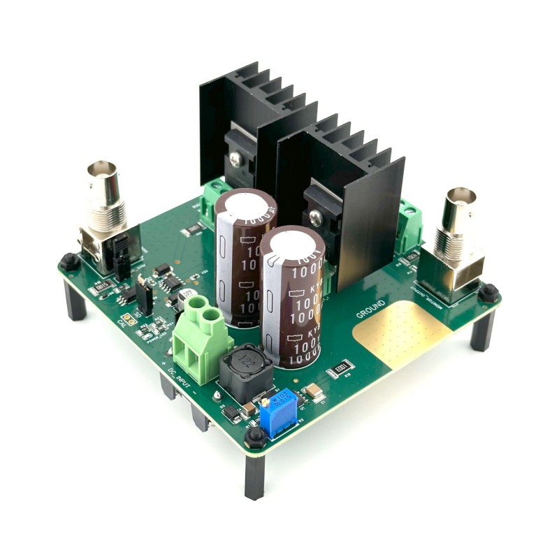
If you are designing a single-switch power stage instead, our standard MOSFET switch board provides the controlled switching device. It leaves the energy-transfer path, reset, current limiting and output control to the surrounding circuit. This makes it useful as a building block when an integrated bridge is not the arrangement you need.
Using a flyback transformer with a voltage multiplier
A Cockcroft–Walton high-voltage multiplier uses a network of diodes and capacitors to produce a DC voltage higher than its input voltage. As the input changes polarity, the diodes direct charge into the capacitors, and the capacitor voltages add to produce the higher output. This design needs AC to keep the charging process going, which makes an unrectified AC flyback transformer a suitable source. Spellman's multiplier explanation describes the operating principle.
Our HVE 10× high-voltage multiplier accepts a maximum AC input of 10 kV peak. For a symmetric waveform, this is 20 kV peak-to-peak; the 10 kV limit is not an RMS rating. When using either AC flyback transformer to supply it, adjust the drive so the voltage at the multiplier input stays within this limit with the intended load connected. The transformer can produce more voltage than the multiplier accepts, so its full output range cannot be used with this module.
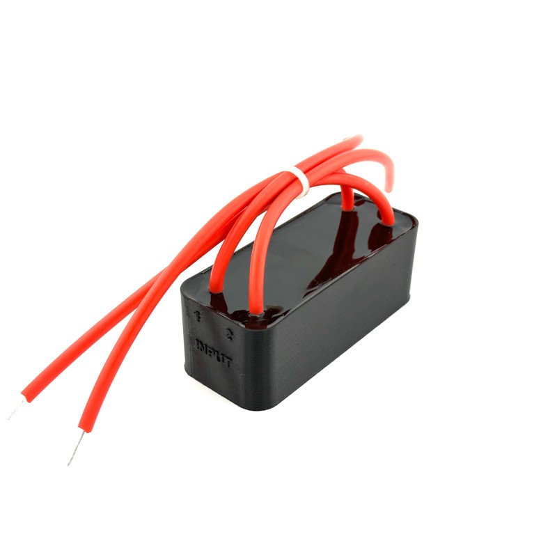
Frequency and current must be matched too. The multiplier's nominal frequency range is 20–300 kHz, which must overlap the transformer's usable range with the module and load connected. Its 50 mA rating applies to the input current, not the high-voltage output current. Because the multiplier also changes the load seen by the transformer, the best operating frequency may shift when it is attached.
Verify the output with the actual load connected
Finally, measure the flyback transformer output voltage with the intended load connected. Record the polarity, peak or peak-to-peak voltage, frequency and temperature together so that the measurement describes the actual operating condition. Remember that the probe becomes part of the circuit: its resistance and capacitance can change a high-impedance output. Tektronix explains this probe-loading effect. Figure 7 shows the difference between an alternating output, rectified pulses and an output with added smoothing capacitance.
Common flyback transformer questions
Can I power a flyback transformer from a DC supply?
Yes. A DC supply can power the switching driver, which then applies changing voltage to the primary. Connecting steady DC directly across the primary does not sustain transformer action after the initial transient. It can saturate the core and cause excessive current, so the driver is an essential part of the circuit.
Can a half-bridge drive a DC flyback transformer?
Yes, if the primary winding and driver are compatible. Check the applied waveform, voltage, frequency and reference connections. The DC label describes the rectified secondary output; the primary still needs a changing voltage. A half-bridge can provide that drive when its operating conditions match the transformer.
Can I get AC from a DC flyback by changing the driver?
Changing the driver does not remove the internal rectifier. If you need access to both secondary voltage polarities, choose a transformer explicitly supplied without an internal diode. Check its winding connections and output reference as part of that choice.
Is a full-bridge always better than a half-bridge?
A full-bridge is useful when the design benefits from applying the full DC bus voltage across the primary. It needs four switches and coordinated timing, and the winding must support the resulting voltage-time stress. A half-bridge may be a simpler choice when its primary voltage is sufficient. Choose the arrangement that provides the required drive within the transformer's operating limits.
Which transformer should I choose for a high-voltage multiplier?
For the Cockcroft–Walton design described above, choose an AC-output transformer without an internal rectifier. Match the loaded output voltage and operating frequency to the multiplier's specifications. Then adjust the drive with the multiplier and intended load connected, since they can change the transformer's resonant response.
Technical references
- Texas Instruments: Voltage Fed Full Bridge DC-DC and DC-AC Converter — push-pull and bridge arrangements, switch voltage and transformer flux balance.
- Analog Devices: MAXREFDES1040 flyback reference design — single-switch energy transfer, reset and MOSFET voltage stress.
- Analog Devices: Parallel LC Resonance — magnetic and electric energy exchange, losses and winding self-resonance.
- Texas Instruments: Measure your LLC resonant tank before testing at full operating conditions — transformer coupling, leakage inductance and additional resonances.
- Coilcraft: Structured Design of Switching Power Transformers — primary turns and voltage-time limits.
- Coilcraft: Measuring Self Resonant Frequency — resonance and measurement loading.
- Spellman: What Is a Voltage Multiplier? — AC-driven diode/capacitor multiplication.
- Tektronix: How Oscilloscope Probes Affect Your Measurement — voltage-probe loading.
- Analog Devices: LTC3721-1 push-pull PWM controller — adjustable frequency, pulse width, dead time and cycle-by-cycle current limiting.
- Texas Instruments: Average Current Limit Balances Center Point of Half-Bridge Input Caps — capacitor charge balance and current-control circuitry.
- Fairchild Semiconductor: AN4136 resonant inverter application note — self-oscillating resonant operation and approximately 50% switching duty.
- Improving Mazzilli’s Driver — the original circuit, gate-drive operation and improvements illustrated with LTspice simulations.
- STMicroelectronics: An introduction to LLC resonant half-bridge converter — resonant operation and overload current.



No comments yet. Be the first to start the conversation.